Clustering using DBSCAN and its extension OPTICS

The goal here is to see if the clusters that we can see in the UMAP are interesting… And as we will see they are not.

import pandas as pd
import numpy as np
from pathlib import Path
import utils

# dimensionality reduction
from sklearn.decomposition import PCA
from umap import umap_ as UMAP

# graphing
import seaborn as sns
import matplotlib.pyplot as plt
import matplotlib.gridspec as gridspec
import plotly.express as px
import plotly.offline as pyo
pyo.init_notebook_mode()
# clustering
from sklearn.cluster import OPTICS, cluster_optics_dbscan

Preprocessing of the data

DATA_PATH = Path.cwd() / "../data"
data = {
    Path(f).stem: pd.read_csv(f, index_col=0) for f in DATA_PATH.glob("combined_*.csv")
}
print(list(data.keys()))

['combined_metrics_finished_edges', 'combined_metrics_finished_paths', 'combined_metrics_unfinished_edges', 'combined_metrics_unfinished_paths']

features_finished_paths = data["combined_metrics_finished_paths"].reset_index(drop=True)
features_unfinished_paths = data["combined_metrics_unfinished_paths"].reset_index(
    drop=True
)
# drop timeout paths
features_unfinished_paths = features_unfinished_paths[features_unfinished_paths["type"] != "timeout"]
features_unfinished_paths

	index	hashedIpAddress	timestamp	durationInSec	path	target	type	backtrack	numberOfPath	path_length	...	ratio	average_time_on_page	sucessive_pairs	sucessive_pairs_encoded	semantic_similarity	path_degree_abs_sum	path_clustering_abs_sum	path_degree_centrality_abs_sum	path_betweenness_abs_sum	path_closeness_abs_sum
4	7	6d136e371e42474f	2011-02-07 18:07:50	175	['4-2-0', 'United_States', 'Agriculture', 'Sug...	Cane_Toad	restart	0	170.0	5	...	3	35.000000	[('4-2-0', 'United_States'), ('United_States',...	[0.19640377163887024, 0.2371780127286911, 0.32...	0.245052	7.585732	-2.590255	-0.846121	-2.271594	-0.927471
7	12	781192ee1a708bec	2011-02-08 03:46:15	334	['Saint_Kitts_and_Nevis', 'United_Kingdom', 'W...	Sandy_Koufax	restart	0	1.0	5	...	3	66.800000	[('Saint_Kitts_and_Nevis', 'United_Kingdom'), ...	[0.48519760370254517, 0.33719098567962646, 0.3...	0.331910	7.578032	-2.211302	-0.853821	-2.267709	-1.553485
9	14	781192ee1a708bec	2011-02-08 03:55:46	403	['Symmetry', 'Science', 'Age_of_Enlightenment'...	Scottish_Episcopal_Church	restart	0	3.0	6	...	1	67.166667	[('Symmetry', 'Science'), ('Science', 'Age_of_...	[0.33117276430130005, 0.20039768517017365, 0.5...	0.336678	6.702728	-3.747010	-1.729125	-3.174033	-2.621027
10	16	5900aa2d71b99153	2011-02-08 04:23:24	115	['Tasmanian_Devil', 'Dog', 'Postage_stamp', 'W...	Love	restart	0	1.0	4	...	3	28.750000	[('Tasmanian_Devil', 'Dog'), ('Dog', 'Postage_...	[0.28771334886550903, 0.27162858843803406, 0.1...	0.246961	4.382027	-1.092701	-4.049827	-6.726992	-2.428974
13	19	2d49dfd2673786bf	2011-02-08 06:47:04	245	['Tim_Berners-Lee', 'England', 'Atlantic_Ocean...	Volcanic_pipe	restart	0	2.0	6	...	3	40.833333	[('Tim_Berners-Lee', 'England'), ('England', '...	[0.10544373840093613, 0.3065592646598816, 0.41...	0.339931	6.422029	-3.488079	-2.009824	-3.429649	-2.719443
...	...	...	...	...	...	...	...	...	...	...	...	...	...	...	...	...	...	...	...	...	...
18974	24867	109ed71f571d86e9	2014-01-15 11:01:43	152	['Montenegro', 'World_War_II', 'United_States'...	Hurricane_Georges	restart	0	20.0	7	...	4	21.714286	[('Montenegro', 'World_War_II'), ('World_War_I...	[0.16399337351322174, 0.3004598617553711, 0.40...	0.463695	6.294228	-2.251847	-2.137626	-3.529575	-2.658404
18975	24868	109ed71f571d86e9	2014-01-15 11:36:08	72	['Wine', 'Georgia_%28country%29', 'Russia']	History_of_post-Soviet_Russia	restart	0	27.0	3	...	2	24.000000	[('Wine', 'Georgia_%28country%29'), ('Georgia_...	[0.12671996653079987, 0.37717318534851074]	0.251947	NaN	NaN	NaN	NaN	NaN
18976	24869	109ed71f571d86e9	2014-01-15 12:00:12	182	['Turks_and_Caicos_Islands', 'United_States', ...	Iraq_War	restart	0	35.0	6	...	2	30.333333	[('Turks_and_Caicos_Islands', 'United_States')...	[0.4149491488933563, 0.40031811594963074, 0.39...	0.421867	7.555088	-1.505405	-0.876766	-2.304742	-1.574654
18977	24870	109ed71f571d86e9	2014-01-15 12:06:45	180	['Franz_Kafka', 'Tuberculosis', 'World_Health_...	Cholera	restart	1	37.0	6	...	3	30.000000	[('Franz_Kafka', 'Tuberculosis'), ('Tuberculos...	[0.2173137068748474, 0.3479086458683014, 0.420...	0.368187	3.669951	-3.305998	-4.761902	-7.644179	-4.383847
18980	24874	1cf0cbb3281049ab	2014-01-15 21:54:01	352	['Mark_Antony', 'Rome', 'Tennis', 'Hawk-Eye', ...	Feather	restart	0	49.0	5	...	2	70.400000	[('Mark_Antony', 'Rome'), ('Rome', 'Tennis'), ...	[0.27006441354751587, 0.28349533677101135, 0.2...	0.237981	5.595124	-1.730546	-2.836729	-5.768889	-2.107167

11811 rows × 24 columns

combined_df = pd.concat([features_finished_paths, features_unfinished_paths], axis=0)
combined_df['finished'] = [1] * len(features_finished_paths) + [0] * len(features_unfinished_paths)
combined_df[utils.FEATURES_COLS_USED_FOR_CLUSTERING] = utils.normalize_features(combined_df[utils.FEATURES_COLS_USED_FOR_CLUSTERING])

X = combined_df[utils.FEATURES_COLS_USED_FOR_CLUSTERING].copy().values
#find number of NaNs in each column
nans = np.isnan(X).sum(axis=0)
print(nans)
#drop rows with NaNs
X = X[~np.isnan(X).any(axis=1)]

[0 0 3 0 0 0 0 0 0 0]

Let’s find the dimensionality of the data

# find the dimensionality of the data
with plt.style.context("dark_background"):
    pca = PCA(n_components=X.shape[1])
    pca.fit(X)
    # plot the explained variance
    plt.scatter(range(1, X.shape[1] + 1), pca.explained_variance_ratio_, c="cyan")
    plt.xlabel("Number of components", fontsize=16)
    plt.ylabel("Explained variance", fontsize=16)
    plt.title("Percentage of explained variance\nof each component of the PCA", fontsize=20)
    plt.show()

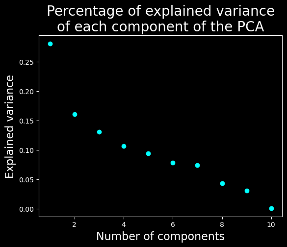
We will keep only the 7 first dimensions

Clustering

We will run optics on a lower dimension to avoid the curse of the dimensionality

Let’s find the latent space using a UMAP

# UMAP
umap = UMAP.UMAP(n_components=7, metric="euclidean")
result_umap_euc = umap.fit_transform(
    X
)

Run the clustering in this space using OPTICS or fixed cutoff values with DBSCAN

#code taken from https://scikit-learn.org/stable/auto_examples/cluster/plot_optics.html
clust = OPTICS(min_samples=50, xi=0.05, min_cluster_size=0.05)

# Run the fit
clust.fit(result_umap_euc)

labels_050 = cluster_optics_dbscan(
    reachability=clust.reachability_,
    core_distances=clust.core_distances_,
    ordering=clust.ordering_,
    eps=0.5,
)
labels_200 = cluster_optics_dbscan(
    reachability=clust.reachability_,
    core_distances=clust.core_distances_,
    ordering=clust.ordering_,
    eps=2,
)

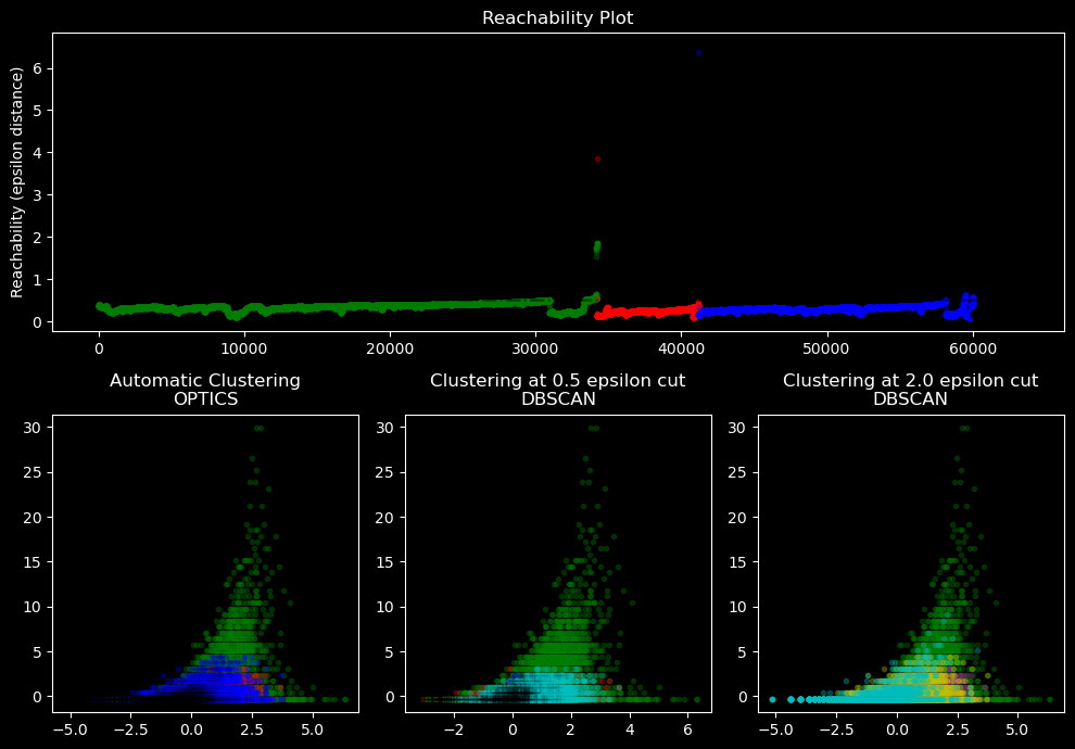
Visualize the results in the plan defined by the 2 first features and draw a reachability plot

space = np.arange(len(X))
reachability = clust.reachability_[clust.ordering_]
labels = clust.labels_[clust.ordering_]

with plt.style.context("dark_background"):
    plt.figure(figsize=(10, 7))
    G = gridspec.GridSpec(2, 3)
    ax1 = plt.subplot(G[0, :])
    ax2 = plt.subplot(G[1, 0])
    ax3 = plt.subplot(G[1, 1])
    ax4 = plt.subplot(G[1, 2])

    # Reachability plot
    colors = ["g.", "r.", "b.", "y.", "c."]
    for klass, color in zip(range(0, 5), colors):
        Xk = space[labels == klass]
        Rk = reachability[labels == klass]
        ax1.plot(Xk, Rk, color, alpha=0.3)
    ax1.plot(space[labels == -1], reachability[labels == -1], "k.", alpha=0.3)
    ax1.plot(space, np.full_like(space, 2.0, dtype=float), "k-", alpha=0.5)
    ax1.plot(space, np.full_like(space, 0.5, dtype=float), "k-.", alpha=0.5)
    ax1.set_ylabel("Reachability (epsilon distance)")
    ax1.set_title("Reachability Plot")

    # OPTICS
    colors = ["g.", "r.", "b.", "y.", "c."]
    for klass, color in zip(range(0, 5), colors):
        Xk = X[clust.labels_ == klass]
        ax2.plot(Xk[:, 0], Xk[:, 1], color, alpha=0.3)
    ax2.plot(X[clust.labels_ == -1, 0], X[clust.labels_ == -1, 1], "k+", alpha=0.1)
    ax2.set_title("Automatic Clustering\nOPTICS")

    # DBSCAN at 0.5
    colors = ["g.", "r.", "b.", "c."]
    for klass, color in zip(range(0, 4), colors):
        Xk = X[labels_050 == klass]
        ax3.plot(Xk[:, 0], Xk[:, 1], color, alpha=0.3)
    ax3.plot(X[labels_050 == -1, 0], X[labels_050 == -1, 1], "k+", alpha=0.1)
    ax3.set_title("Clustering at 0.5 epsilon cut\nDBSCAN")

    # DBSCAN at 2.
    colors = ["g.", "m.", "y.", "c."]
    for klass, color in zip(range(0, 4), colors):
        Xk = X[labels_200 == klass]
        ax4.plot(Xk[:, 0], Xk[:, 1], color, alpha=0.3)
    ax4.plot(X[labels_200 == -1, 0], X[labels_200 == -1, 1], "k+", alpha=0.1)
    ax4.set_title("Clustering at 2.0 epsilon cut\nDBSCAN")

    plt.tight_layout()
    plt.show()

Create a UMAP with 3 dimensions for visualization purposes

from umap import umap_ as UMAP
# UMAP
umap = UMAP.UMAP(n_components=3, metric="euclidean")
result_umap_euc = umap.fit_transform(
    X
)

fig = px.scatter_3d(
    result_umap_euc,
    x=0,
    y=1,
    z=2,
    color=clust.labels_.astype(str),
    title="UMAP, showing OPTICS clustering",
    # reduce size points
    size_max=0.1,
    category_orders={"color": [str(i) for i in range(0, len(np.unique(clust.labels_)))]},
)
fig.update_layout({"plot_bgcolor": "#14181e", "paper_bgcolor": "#14181e"})
fig.update_layout(font_color="white")
fig.update_layout(scene=dict(xaxis=dict(showticklabels=False), yaxis=dict(showticklabels=False), zaxis=dict(showticklabels=False)))
fig.update_layout(legend_title_text="Cluster")
fig.update_layout(legend = dict(bgcolor = 'rgba(0,0,0,0)'))
fig.update_layout(scene=dict(xaxis_title="UMAP 1", yaxis_title="UMAP 2", zaxis_title="UMAP 3"))
fig.update_layout(scene = dict(
    xaxis = dict(
            backgroundcolor="rgba(0, 0, 0,0)",
            # gridcolor="rgba(0, 0, 0,0)", # gridcolor is for logo
            showbackground=True,
            zerolinecolor="white",),
    yaxis = dict(
        backgroundcolor="rgba(0, 0, 0,0)",
        # gridcolor="rgba(0, 0, 0,0)",
        showbackground=True,
        zerolinecolor="white"),
    zaxis = dict(
        backgroundcolor="rgba(0, 0, 0,0)",
        # gridcolor="rgba(0, 0, 0,0)",
        showbackground=True,
        zerolinecolor="white",),),
)
display(fig)

By providing a UMAP in 7 dimension to OPTICS we roughly find the communities that we can see by eye in the 3D UMAP

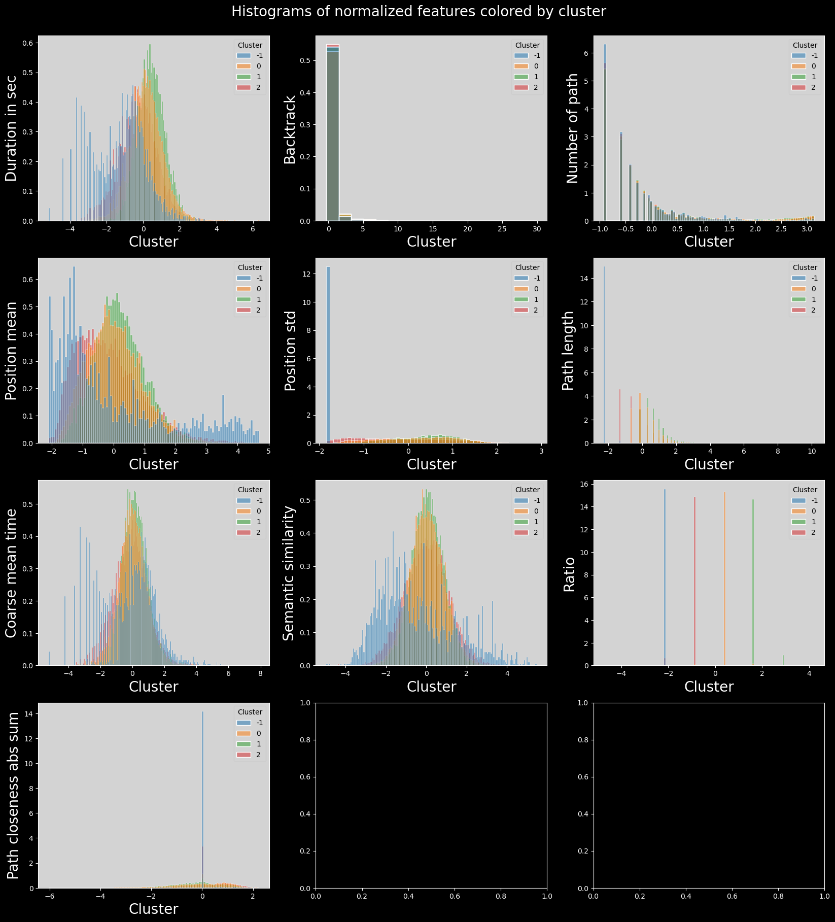
Visualization of the results

#plot histogram features colored by cluster
with plt.style.context("dark_background"):
    plot_data = combined_df[utils.FEATURES_COLS_USED_FOR_CLUSTERING].copy().dropna()
    plot_data["cluster"] = clust.labels_
    plot_data["cluster"] = plot_data["cluster"].astype("category")
    n_features = len(plot_data.columns) - 1
    n_cols = 3
    n_rows = int(np.ceil(n_features / n_cols))
    fig, axs = plt.subplots(n_rows, n_cols, figsize=(20, 20))
    axs = axs.flatten()
    for i, col in enumerate(plot_data.columns):
        if col == "cluster":
            continue
        sns.histplot(
            data=plot_data,
            x=col,
            hue="cluster",
            ax=axs[i],
            stat="density",
            common_norm=False,
            palette="tab10",
        )
        utils.set_axis_style(axs, i)

    plt.suptitle("Histograms of normalized features colored by cluster", fontsize=20)
    plt.subplots_adjust(top=0.95)
    plt.show()

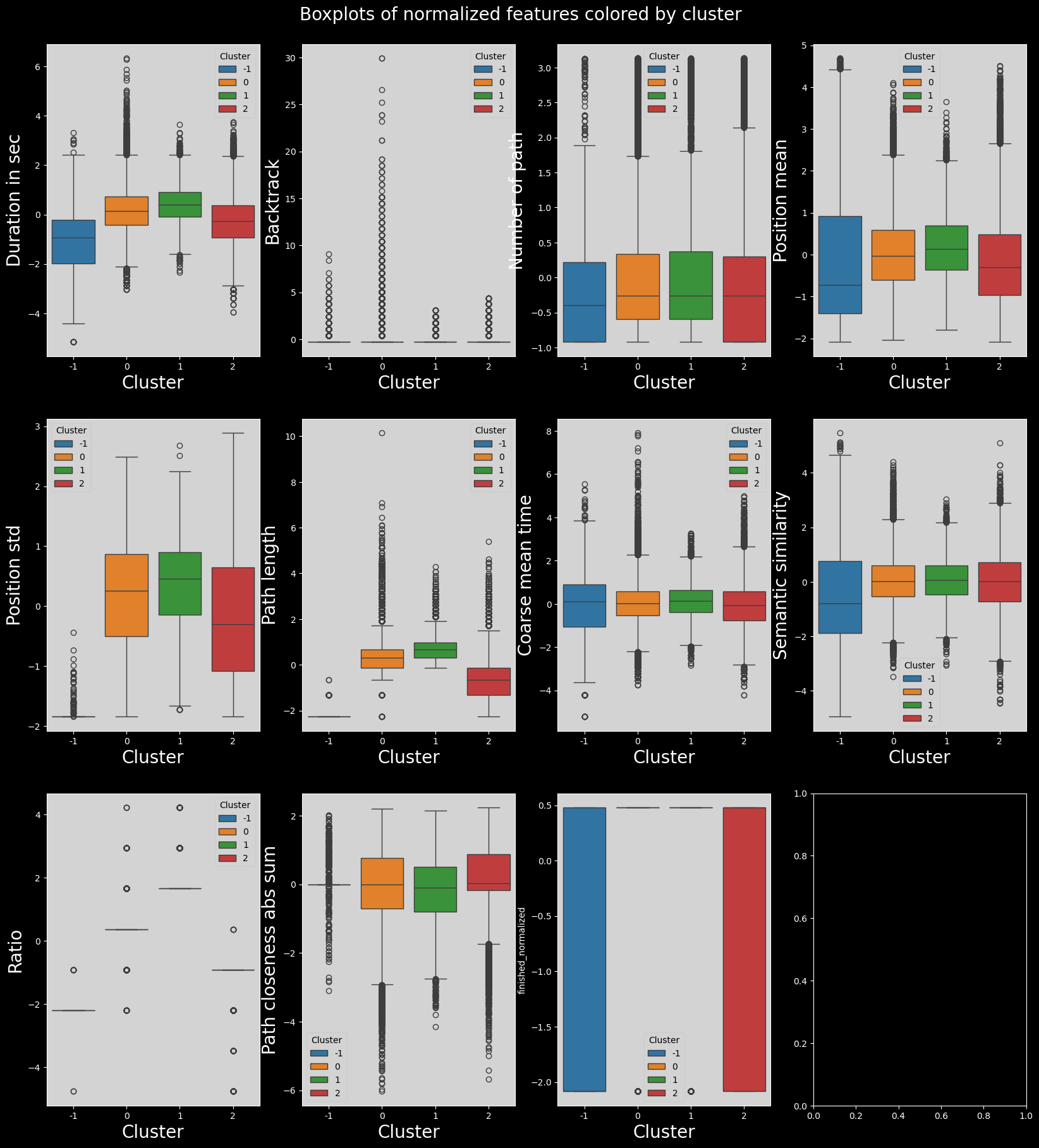
with plt.style.context("dark_background"):
    combined_df = combined_df[utils.FEATURES_COLS_USED_FOR_CLUSTERING+["finished"]].dropna()
    combined_df["finished_normalized"] = (
        combined_df["finished"] - combined_df["finished"].mean()
    ) / combined_df["finished"].std()
    plot_data = combined_df[utils.FEATURES_COLS_USED_FOR_CLUSTERING + ["finished_normalized"]].copy()
    plot_data["cluster"] = clust.labels_
    plot_data["cluster"] = plot_data["cluster"].astype("category")
    n_features = len(plot_data.columns) - 1
    n_cols = 4
    n_rows = int(np.ceil(n_features / n_cols))
    fig, axs = plt.subplots(n_rows, n_cols, figsize=(20, 20))
    fig.suptitle("Boxplots of normalized features colored by cluster", fontsize=20)
    plt.subplots_adjust(top=0.95)
    axs = axs.flatten()
    for i, col in enumerate(plot_data.columns):
        if col == "cluster":
            continue
        sns.boxplot(data=plot_data, x="cluster", y=col, ax=axs[i], hue="cluster", palette="tab10")
        utils.set_axis_style(axs, i)
    plt.show()

# heatmap of features means per cluster
feat_labels = utils.get_feature_names_labels()
with plt.style.context("dark_background"):
    means = plot_data.groupby(plot_data["cluster"]).mean()
    sns.heatmap(means, cmap="coolwarm", annot=True, fmt=".1f", vmin=-1, vmax=1)
    plt.title("Heatmap of normalized features\nmeans per cluster", fontsize=25)
    plt.ylabel("Cluster", fontsize=20)
    plt.xlabel("Feature", fontsize=20)
    plt.xticks(labels=feat_labels+["Finished (norm)"], ticks=np.arange(len(feat_labels)+1)+0.5, rotation=90, fontsize=15)
    plt.show()

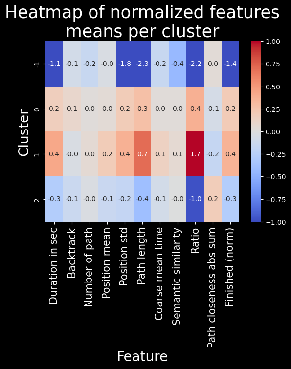
Discussion and conclusion

Here we can see that the clustering is less interesting. It really makes 4 clusters in which all the features used to do the clustering are either very low, low, high or very high.