Alternative clustering methods

Alternative methods overview

In this section, we show two different clustering methods which were used on top of Leiden clustering (our preferred method).

These two methods are agglomerative clustering (hierarchical clustering) and gaussian mixture model-based (GMM) clustering. We show that these methods are not as good as Leiden clustering.

Agglomerative clustering

Agglomerative clustering is a hierarchical clustering method. It starts with each point in its own cluster and then merges the two closest clusters iteratively until there is only one cluster left. We use the Euclidean distance as the distance metric, with ward linkage (cluster linkage which minimises intra-cluster variance), which was by far the best mon linkage methods tried. We use the AgglomerativeClustering class from sklearn.cluster to perform agglomerative clustering.

Gaussian mixture model-based clustering

Gaussian mixture model-based clustering is a clustering method which assumes that the data is generated from a mixture of Gaussian distributions. We use the GaussianMixture class from sklearn.mixture to perform Gaussian mixture model-based clustering.

Data loading and preprocessing

import pandas as pd
import numpy as np
import seaborn as sns
import matplotlib.pyplot as plt
from pathlib import Path
import utils
import sklearn.cluster
import sklearn.mixture
import numpy as np
from scipy.cluster.hierarchy import dendrogram
from sklearn.decomposition import PCA
from sklearn.manifold import TSNE
from umap import umap_ as umap
import plotly.express as px
import plotly.offline as pyo

pyo.init_notebook_mode()

DATA_PATH = Path.cwd() / "../data"
data = {
    Path(f).stem: pd.read_csv(f, index_col=0) for f in DATA_PATH.glob("combined_*.csv")
}
print(list(data.keys()))

['combined_metrics_finished_edges', 'combined_metrics_finished_paths', 'combined_metrics_unfinished_edges', 'combined_metrics_unfinished_paths']

features_finished_paths = data["combined_metrics_finished_paths"].reset_index(drop=True)
features_unfinished_paths = data["combined_metrics_unfinished_paths"].reset_index(
    drop=True
)
features_used=utils.FEATURES_COLS_USED_FOR_CLUSTERING

combined_df = pd.concat([features_finished_paths, features_unfinished_paths], axis=0)
combined_df['finished'] = [1] * len(features_finished_paths) + [0] * len(features_unfinished_paths)
combined_df[features_used] = utils.normalize_features(combined_df[utils.FEATURES_COLS_USED_FOR_CLUSTERING])
X = combined_df[features_used].values
#find number of NaNs in each column
nans = np.isnan(X).sum(axis=0)
print(nans)
#drop rows with NaNs
mask_vector = ~np.isnan(X).any(axis=1)
X = X[~np.isnan(X).any(axis=1)]

[0 0 3 0 0 0 0 0 0 0]

# drop the path sum metrics
combined_df

	hashedIpAddress	timestamp	durationInSec	path	rating	backtrack	numberOfPath	path_length	coarse_mean_time	position_mean	...	semantic_similarity	path_degree_abs_sum	path_clustering_abs_sum	path_degree_centrality_abs_sum	path_betweenness_abs_sum	path_closeness_abs_sum	index	target	type	finished
0	6a3701d319fc3754	2011-02-15 03:26:49	0.094978	['14th_century', '15th_century', '16th_century...	NaN	-0.280785	-0.360322	1.237829	-0.293402	0.011529	...	1.882018	5.197422	-3.233355	-3.234431	-5.004633	-0.430555	NaN	NaN	NaN	1
1	3824310e536af032	2012-08-12 06:36:52	-0.422557	['14th_century', 'Europe', 'Africa', 'Atlantic...	3.0	-0.280785	0.358481	-0.067835	-0.333922	-0.627881	...	1.190749	7.010212	-2.318889	-1.421642	-3.524030	0.953234	NaN	NaN	NaN	1
2	415612e93584d30e	2012-10-03 21:10:40	-0.055666	['14th_century', 'Niger', 'Nigeria', 'British_...	NaN	-0.280785	0.544508	0.976194	-0.351290	-0.369856	...	0.770837	5.236336	-3.212821	-3.195518	-4.962358	-0.403703	NaN	NaN	NaN	1
3	64dd5cd342e3780c	2010-02-08 07:25:25	-1.129090	['14th_century', 'Renaissance', 'Ancient_Greec...	NaN	-0.280785	-0.559082	-0.563509	-0.890117	-0.442103	...	0.535863	NaN	NaN	NaN	NaN	0.000000	NaN	NaN	NaN	1
4	015245d773376aab	2013-04-23 15:27:08	0.138033	['14th_century', 'Italy', 'Roman_Catholic_Chur...	3.0	-0.280785	-0.898865	0.679578	-0.030457	0.062407	...	-0.815607	6.315864	-2.737924	-2.115989	-4.991059	0.562986	NaN	NaN	NaN	1
...	...	...	...	...	...	...	...	...	...	...	...	...	...	...	...	...	...	...	...	...	...
18976	109ed71f571d86e9	2014-01-15 12:00:12	0.170016	['Turks_and_Caicos_Islands', 'United_States', ...	NaN	-0.280785	0.843977	0.337160	0.136738	0.774194	...	0.089435	7.555088	-1.505405	-0.876766	-2.304742	1.021614	24869.0	Iraq_War	restart	0
18977	109ed71f571d86e9	2014-01-15 12:06:45	0.161005	['Franz_Kafka', 'Tuberculosis', 'World_Health_...	NaN	0.337716	0.871218	0.337160	-0.121555	-0.310926	...	-0.462655	3.669951	-3.305998	-4.761902	-7.644179	-1.914494	24870.0	Cholera	restart	0
18978	2e09a7224600a7cd	2014-01-15 15:06:40	2.082769	['Computer_programming', 'Linguistics', 'Cultu...	NaN	0.337716	-0.109914	-1.202543	2.322458	1.156748	...	-0.102215	4.760035	-2.802979	-3.671818	-6.478384	0.412224	24872.0	The_Beatles	timeout	0
18979	60af9e2138051b96	2014-01-15 15:24:41	2.084055	['Jamaica', 'United_Kingdom', 'World_War_II', ...	NaN	-0.280785	-0.898865	-0.563509	2.516759	-1.107312	...	-0.259947	7.158709	-1.836719	-1.273145	-2.951980	0.864835	24873.0	Alan_Turing	timeout	0
18980	1cf0cbb3281049ab	2014-01-15 21:54:01	0.707915	['Mark_Antony', 'Rome', 'Tennis', 'Hawk-Eye', ...	NaN	-0.280785	1.008917	-0.067835	0.864710	0.666220	...	-1.801801	5.595124	-1.730546	-2.836729	-5.768889	0.465042	24874.0	Feather	restart	0

70290 rows × 26 columns

Finding the dimensionality of the data will not be reiterated here, please refer to the Leiden clustering notebook for more details.

We will keep only the 7 first dimensions.

pca = PCA(n_components=7, random_state=42)
X_pca = pca.fit_transform(X)

Hierarchical clustering

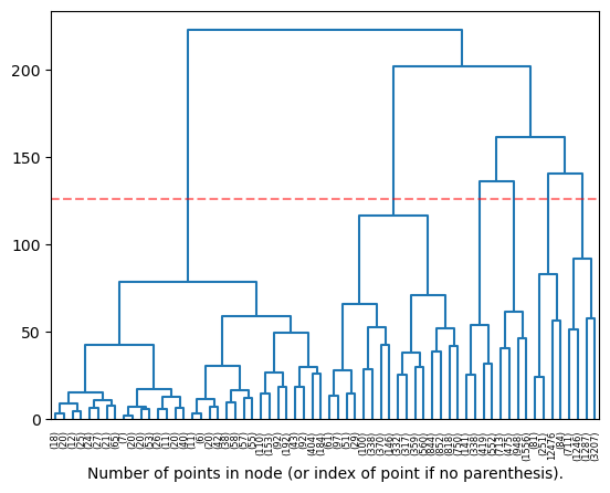
The code below defines the denedogram plotting function, which is used to visualise the decision tree of the hierarchical clustering.

Setup

def plot_dendrogram(model, n_clust, **kwargs): # From sklearn plot clustering dendogram docs: https://scikit-learn.org/stable/auto_examples/cluster/plot_agglomerative_dendrogram.html
    # Create linkage matrix and then plot the dendrogram

    # create the counts of samples under each node
    counts = np.zeros(model.children_.shape[0])
    n_samples = len(model.labels_)
    for i, merge in enumerate(model.children_):
        current_count = 0
        for child_idx in merge:
            if child_idx < n_samples:
                current_count += 1  # leaf node
            else:
                current_count += counts[child_idx - n_samples]
        counts[i] = current_count

    linkage_matrix = np.column_stack(
        [model.children_, model.distances_, counts]
    ).astype(float)

    # Plot the corresponding dendrogram
    dendrogram(linkage_matrix, **kwargs)

    # Draw a line at the threshold (which is derived from the number of clusters)
    plt.axhline(y=(linkage_matrix[-n_clust, 2] + linkage_matrix[-n_clust + 1, 2]) / 2, c='r', linestyle='--', alpha=0.5)

    plt.xlabel("Number of points in node (or index of point if no parenthesis).")
    plt.show()

X_pca.shape

(70287, 7)

Visualisation of the hierarchical clustering

Here we plot a dendrogram of the clustering, and the resulting clusters (on a 3D projection of the data)

# Select a random subset of samples
SUBSAMPLE_SIZE = 20000

np.random.seed(42)
subset_indices = np.random.choice(X_pca.shape[0], size=SUBSAMPLE_SIZE, replace=True)
X_subset = X_pca[subset_indices]
NUM_CLUSTERS = 6

# Run hierarchical clustering on the subset of data (maximum distance between clusters)
model = sklearn.cluster.AgglomerativeClustering(n_clusters=NUM_CLUSTERS, compute_full_tree=True, compute_distances=True, linkage='ward')
Z = model.fit_predict(X_subset)

plot_dendrogram(model, truncate_mode='level', p=5, n_clust=NUM_CLUSTERS, color_threshold=0)

UMAP plot

# umap the data down to 3 dimensions
reducer = umap.UMAP(random_state=42, n_components=3, init='random')
# reducer = PCA(n_components=2, random_state=42)
# reducer = TSNE(n_components=2, random_state=42)
X_umap = reducer.fit_transform(X_subset)

fig = px.scatter_3d(
	x=X_umap[:, 0],
	y=X_umap[:, 1],
	z=X_umap[:, 2],
	color=model.labels_,
	opacity=0.8,
	labels={"color": "cluster"},
	title=f"UMAP of agglomerative clustering of {SUBSAMPLE_SIZE} samples",
)
utils.format_3d_plot(fig)
display(fig)

c:\Users\Cyril\anaconda3\envs\DLbiomed\lib\site-packages\umap\umap_.py:1943: UserWarning:

n_jobs value -1 overridden to 1 by setting random_state. Use no seed for parallelism.

c:\Users\Cyril\anaconda3\envs\DLbiomed\lib\site-packages\pynndescent\pynndescent_.py:346: NumbaPendingDeprecationWarning:

Code using Numba extension API maybe depending on 'old_style' error-capturing, which is deprecated and will be replaced by 'new_style' in a future release. See details at https://numba.readthedocs.io/en/latest/reference/deprecation.html#deprecation-of-old-style-numba-captured-errors
Exception origin:
  File "c:\Users\Cyril\anaconda3\envs\DLbiomed\lib\site-packages\numba\core\types\functions.py", line 486, in __getnewargs__
    raise ReferenceError("underlying object has vanished")


c:\Users\Cyril\anaconda3\envs\DLbiomed\lib\site-packages\pynndescent\pynndescent_.py:348: NumbaPendingDeprecationWarning:

Code using Numba extension API maybe depending on 'old_style' error-capturing, which is deprecated and will be replaced by 'new_style' in a future release. See details at https://numba.readthedocs.io/en/latest/reference/deprecation.html#deprecation-of-old-style-numba-captured-errors
Exception origin:
  File "c:\Users\Cyril\anaconda3\envs\DLbiomed\lib\site-packages\numba\core\types\functions.py", line 486, in __getnewargs__
    raise ReferenceError("underlying object has vanished")


c:\Users\Cyril\anaconda3\envs\DLbiomed\lib\site-packages\pynndescent\pynndescent_.py:358: NumbaPendingDeprecationWarning:

Code using Numba extension API maybe depending on 'old_style' error-capturing, which is deprecated and will be replaced by 'new_style' in a future release. See details at https://numba.readthedocs.io/en/latest/reference/deprecation.html#deprecation-of-old-style-numba-captured-errors
Exception origin:
  File "c:\Users\Cyril\anaconda3\envs\DLbiomed\lib\site-packages\numba\core\types\functions.py", line 486, in __getnewargs__
    raise ReferenceError("underlying object has vanished")

# reducer = umap.UMAP(random_state=42, n_components=2, init='random')
# reducer = PCA(n_components=2, random_state=42)
reducer = TSNE(n_components=3, random_state=42)
X_umap = reducer.fit_transform(X_subset)

t-SNE plot

fig2=px.scatter_3d(
	x=X_umap[:, 0],
	y=X_umap[:, 1],
	z=X_umap[:, 2],
	color=model.labels_.astype(str),
	opacity=0.8,
	labels={"color": "cluster"},
	title=f"TSNE of agglomerative clustering of {SUBSAMPLE_SIZE} samples",
)
utils.format_3d_plot(fig2)
fig.update_layout(scene=dict(xaxis_title="t-SNE 1", yaxis_title="t-SNE 2", zaxis_title="t-SNE 3"))
display(fig)

One can observe that the clustering obtained from this method follows the UMAP and TSNE projections (position in space determines cluster). One of the selected clusters only has 3 points, which is definitely not what we want! (See second line crossing threshold from left.)

Feature distributions per cluster

with plt.style.context("dark_background"):
    plot_data = combined_df[utils.FEATURES_COLS_USED_FOR_CLUSTERING].copy().dropna().iloc[subset_indices]
    plot_data["cluster"] = model.labels_
    plot_data["cluster"] = plot_data["cluster"].astype("category")
    n_features = len(plot_data.columns) - 1
    n_cols = 3
    n_rows = int(np.ceil(n_features / n_cols))
    fig, axs = plt.subplots(n_rows, n_cols, figsize=(20, 20))
    axs = axs.flatten()
    for i, col in enumerate(plot_data.columns):
        if col == "cluster":
            continue
        sns.histplot(
            data=plot_data,
            x=col,
            hue="cluster",
            ax=axs[i],
            stat="density",
            common_norm=False,
            palette="tab10",
        )
        utils.set_axis_style(axs, i)

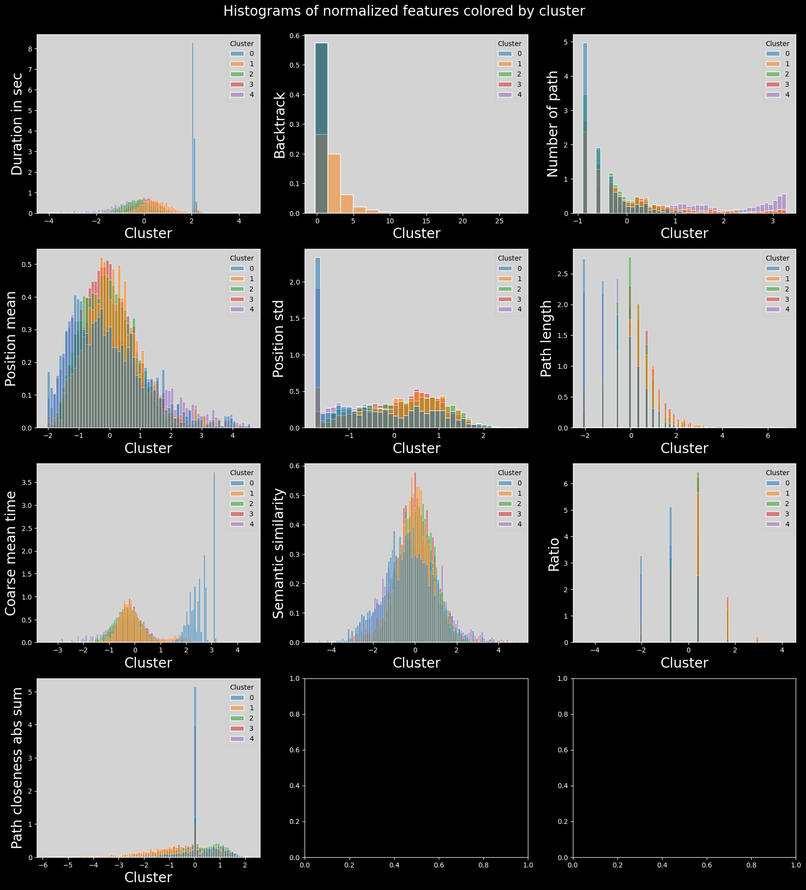
    plt.suptitle("Histograms of normalized features colored by cluster", fontsize=20)
    plt.subplots_adjust(top=0.95)
    plt.show()

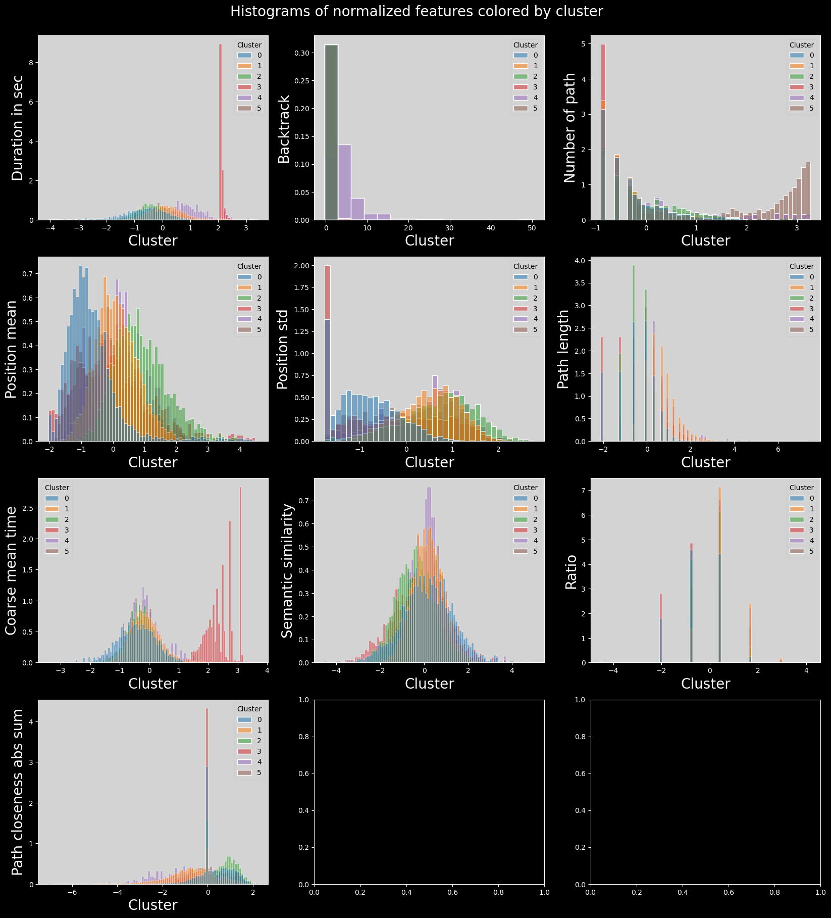
Firstly, these clusters have been computed on a subset, due to memory limitations of the method. Secondly, the clusters are not as well defined as the ones obtained from Leiden clustering. One can observe the presence of significant outliers in the 5th cluster, and very similar values for the rest.

with plt.style.context("dark_background"):
	combined_df["finished_normalized"] = (
		combined_df["finished"] - combined_df["finished"].mean()
	) / combined_df["finished"].std()
	plot_data = combined_df[utils.FEATURES_COLS_USED_FOR_CLUSTERING + ["finished_normalized"]].copy().iloc[subset_indices]

	plot_data.index = np.arange(len(plot_data))

	plot_data["cluster"] = model.labels_

	plot_data["cluster"] = plot_data["cluster"].astype("category")
	n_features = len(plot_data.columns) - 1
	n_cols = 4
	n_rows = int(np.ceil(n_features / n_cols))
	fig, axs = plt.subplots(n_rows, n_cols, figsize=(20, 20))
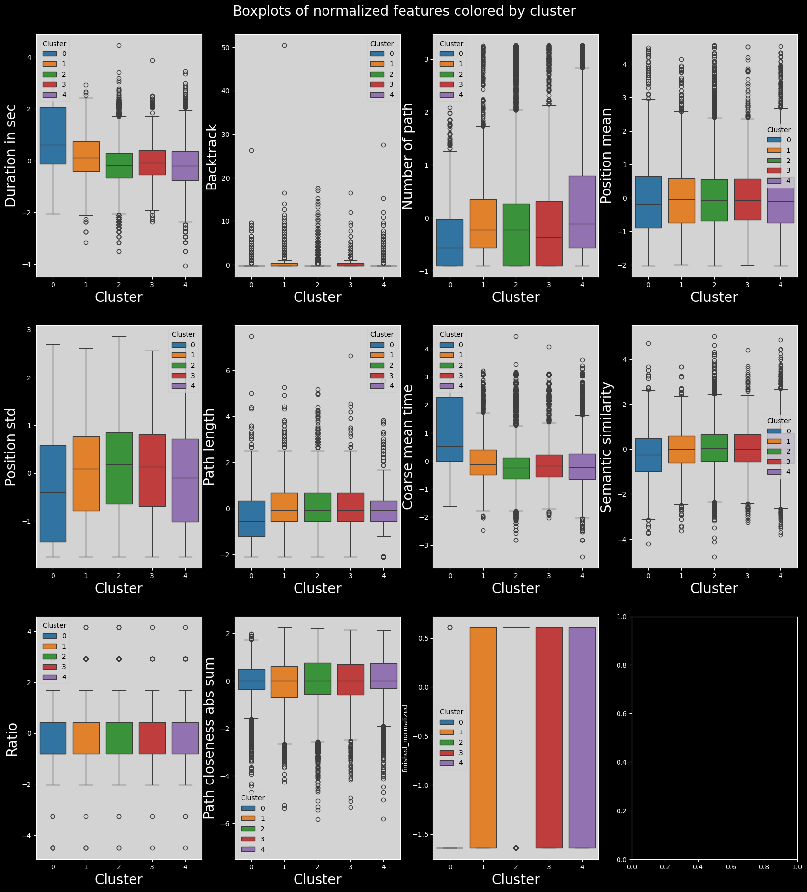
	fig.suptitle("Boxplots of normalized features colored by cluster", fontsize=20)
	plt.subplots_adjust(top=0.95)
	axs = axs.flatten()
	for i, col in enumerate(plot_data.columns):
		if col == "cluster":
			continue
		sns.boxplot(data=plot_data, x="cluster", y=col, ax=axs[i], hue="cluster", palette="tab10")
		utils.set_axis_style(axs, i)
	plt.show()

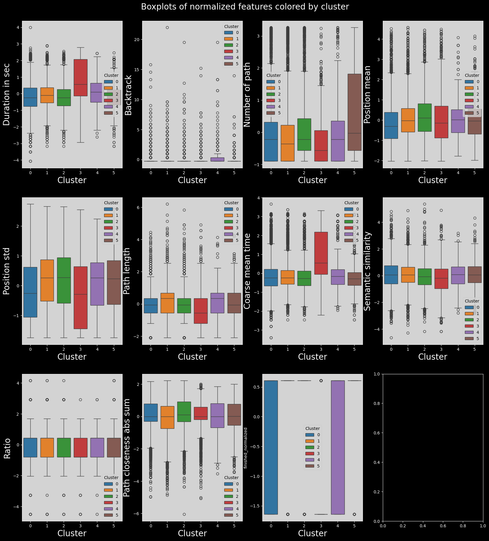
A lot of features do not vary by cluster. This is not wanted behaviour, as we want to find features which vary by cluster.

clusters_names,n_points = np.unique(plot_data["cluster"], return_counts=True)
with plt.style.context("dark_background"):
    sns.barplot(x=clusters_names, y=n_points,hue=range(len(clusters_names)), palette="tab10").set_title("Number of paths per cluster", fontsize=20)
    # make background grey
    plt.gca().patch.set_facecolor("#d3d3d3")
    # update legend style
    leg = plt.gca().get_legend()
    leg.get_frame().set_facecolor("#d3d3d3")
    leg.set_title("Cluster")
    leg_title = leg.get_title()
    leg_title.set_color("black")
    # change all legend text to black
    [text.set_color("black") for text in leg.get_texts()]
    plt.xlabel("Cluster", fontsize=14)
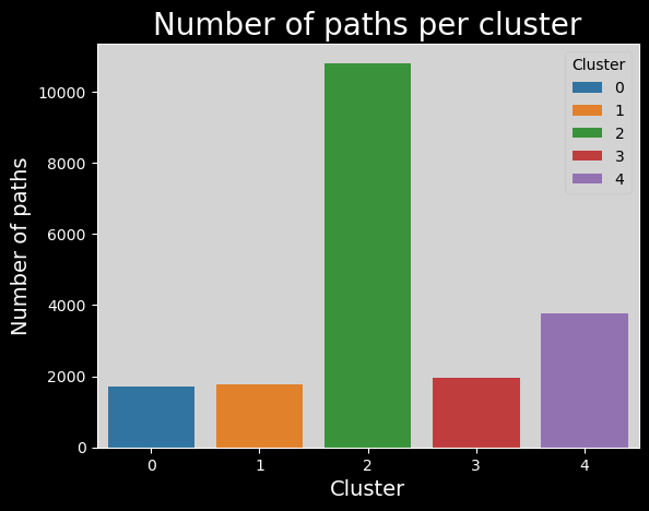
    plt.ylabel("Number of paths", fontsize=14)
plt.show()

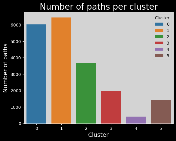
This is a relatively nice distribution.

analysis_df = combined_df.copy().iloc[subset_indices]
analysis_df['cluster'] = Z

feat_labels = utils.get_feature_names_labels()
with plt.style.context("dark_background"):
    means = plot_data.groupby(plot_data["cluster"]).mean()
    sns.heatmap(means, cmap="coolwarm", annot=True, fmt=".1f", vmin=-1, vmax=1)
    plt.title("Heatmap of normalized features\nmeans per cluster", fontsize=25)
    plt.ylabel("Cluster", fontsize=20)
    plt.xlabel("Feature", fontsize=20)
    plt.xticks(labels=feat_labels+["Finished (norm)"], ticks=np.arange(len(feat_labels)+1)+0.5, rotation=90, fontsize=15)
    plt.show()

Here, interestingly enough, we can sort of identify player behaviour through these clusters.

1. Cluster 5 comprises players which are more often on longer paths. These players are likely experienced and capable of finishing more on average.

2. Cluster 3 comprises player which struggle more with completing the task: they take longer, take less optimal paths, and often do not finish.

3. Clusters 0, 1, 2, and 4 are too related to distinguish.

In the end, unfortunately, these clusters are not very interesting.

Gaussian mixed-model clustering

Visualisation

import numpy as np
# Select a random subset of samples
np.random.seed(42)
subset_indices = np.random.choice(X_pca.shape[0], size=SUBSAMPLE_SIZE, replace=False)
X_subset = X_pca[subset_indices]

# Run hierarchical clustering on the subset of data
model = sklearn.mixture.GaussianMixture(n_components=5)
Z = model.fit_predict(X_subset)

reducer = umap.UMAP(random_state=42, n_components=3, init='random')
X_umap = reducer.fit_transform(X_subset)

c:\Users\Cyril\anaconda3\envs\DLbiomed\lib\site-packages\umap\umap_.py:1943: UserWarning:

n_jobs value -1 overridden to 1 by setting random_state. Use no seed for parallelism.

fig = px.scatter_3d(
	x=X_umap[:, 0],
	y=X_umap[:, 1],
	z=X_umap[:, 2],
	color=Z.astype(str),
	opacity=0.8,
	labels={"color": "cluster"},
	title=f"Gaussian Mixture clustering of {SUBSAMPLE_SIZE} samples",
)
utils.format_3d_plot(fig)
display(fig)

with plt.style.context("dark_background"):
    plot_data = combined_df[utils.FEATURES_COLS_USED_FOR_CLUSTERING].copy().dropna().iloc[subset_indices]
    plot_data["cluster"] = Z
    plot_data["cluster"] = plot_data["cluster"].astype("category")
    n_features = len(plot_data.columns) - 1
    n_cols = 3
    n_rows = int(np.ceil(n_features / n_cols))
    fig, axs = plt.subplots(n_rows, n_cols, figsize=(20, 20))
    axs = axs.flatten()
    for i, col in enumerate(plot_data.columns):
        if col == "cluster":
            continue
        sns.histplot(
            data=plot_data,
            x=col,
            hue="cluster",
            ax=axs[i],
            stat="density",
            common_norm=False,
            palette="tab10",
        )
        utils.set_axis_style(axs, i)

    plt.suptitle("Histograms of normalized features colored by cluster", fontsize=20)
    plt.subplots_adjust(top=0.95)
    plt.show()

with plt.style.context("dark_background"):
	combined_df["finished_normalized"] = (
		combined_df["finished"] - combined_df["finished"].mean()
	) / combined_df["finished"].std()
	plot_data = combined_df[utils.FEATURES_COLS_USED_FOR_CLUSTERING + ["finished_normalized"]].copy().iloc[subset_indices]

	plot_data.index = np.arange(len(plot_data))

	plot_data["cluster"] = Z

	plot_data["cluster"] = plot_data["cluster"].astype("category")
	n_features = len(plot_data.columns) - 1
	n_cols = 4
	n_rows = int(np.ceil(n_features / n_cols))
	fig, axs = plt.subplots(n_rows, n_cols, figsize=(20, 20))
	fig.suptitle("Boxplots of normalized features colored by cluster", fontsize=20)
	plt.subplots_adjust(top=0.95)
	axs = axs.flatten()
	for i, col in enumerate(plot_data.columns):
		if col == "cluster":
			continue
		sns.boxplot(data=plot_data, x="cluster", y=col, ax=axs[i], hue="cluster", palette="tab10")
		utils.set_axis_style(axs, i)
	plt.show()

clusters_names,n_points = np.unique(plot_data["cluster"], return_counts=True)
with plt.style.context("dark_background"):
    sns.barplot(x=clusters_names, y=n_points,hue=range(len(clusters_names)), palette="tab10").set_title("Number of paths per cluster", fontsize=20)
    # make background grey
    plt.gca().patch.set_facecolor("#d3d3d3")
    # update legend style
    leg = plt.gca().get_legend()
    leg.get_frame().set_facecolor("#d3d3d3")
    leg.set_title("Cluster")
    leg_title = leg.get_title()
    leg_title.set_color("black")
    # change all legend text to black
    [text.set_color("black") for text in leg.get_texts()]
    plt.xlabel("Cluster", fontsize=14)
    plt.ylabel("Number of paths", fontsize=14)
plt.show()

We encounter the same problem as before, but slightly different. Instead of one cluster being way too small, we have one cluster that is much too large here!

feat_labels = utils.get_feature_names_labels()
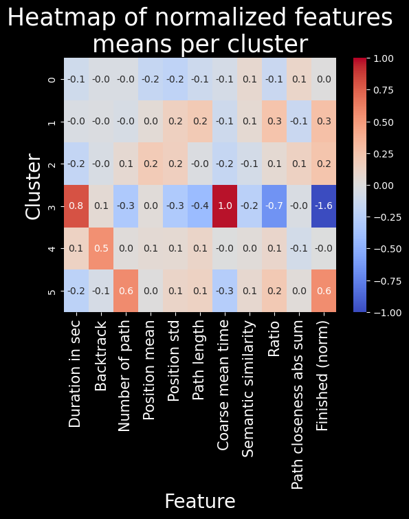
with plt.style.context("dark_background"):
    means = plot_data.groupby(plot_data["cluster"]).mean()
    sns.heatmap(means, cmap="coolwarm", annot=True, fmt=".1f", vmin=-1, vmax=1)
    plt.title("Heatmap of normalized features\nmeans per cluster", fontsize=25)
    plt.ylabel("Cluster", fontsize=20)
    plt.xlabel("Feature", fontsize=20)
    plt.xticks(labels=feat_labels+["Finished (norm)"], ticks=np.arange(len(feat_labels)+1)+0.5, rotation=90, fontsize=15)
    plt.show()

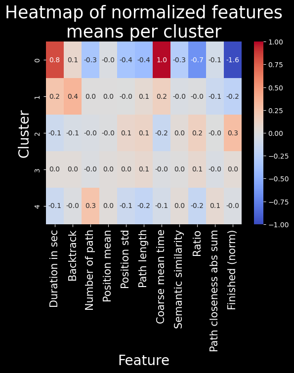
The problem with this clustering method is that due to soft clustering assignment, clusters are a “blur” of sorts, and therefore the differences between them are much less pronounced. This is indeed the case, these clusters are present, but they don’t show us anything!! A single interesting cluster is found, but it’s the same as with hierarchical clustering, so there’s no point in using this method.

---

Conclusion

Due to the fact that we’ve shown that these clustering methods are inferior to Leiden clustering, we will not be performing any statistical clustering analysis, nor continuing with the use of these methods.