MUTAG Dataset

In this homework we will be working with the MUTAG dataset, a graph classification task where we aim to determine if a molecule is mutagenic or not.

Loading the data

We simply use the Hugging Face API to retrieve the dataset; we will save it as a pickle for convenience.

Show code cell source Hide code cell source

%load_ext autoreload
%autoreload 2

Show code cell source Hide code cell source

import sys
import numpy as np
import seaborn as sns
import matplotlib.pyplot as plt
sys.path.append("../code")
import utils

dataset_hf = utils.load_dataset_mutag("./data/mutag.pickle")
dataset_hf

DatasetDict({
    train: Dataset({
        features: ['edge_index', 'node_feat', 'edge_attr', 'y', 'num_nodes'],
        num_rows: 188
    })
})

We see that the dataset consists of 188 graphs, each with certain attributes.

We have :

• node_attr : the node attributes, which represent the atom types in a one-hot encoded format.

• edge_attr : the edge attributes, which are the bond types, also one-hot encoded.

• edge_index : the edge indices, which are the connections between the nodes. This specifies all the from/to connections (edges).

• y : the target, which is a binary label indicating whether the molecule is mutagenic or not.

• num_nodes : the number of nodes in the graph. Can technically be inferred from edge_index.

dataset_hf.shape

{'train': (188, 5)}

edge_indices = dataset_hf["train"]["edge_index"] # contains lists of edges. first dim is the index of a node, e.g. 0, and it will appear as many times as it has edges. second dim is the index of the node it is connected to, e.g. 1
node_features = dataset_hf["train"]["node_feat"] # features of each node, as N_NODES x N_FEATURES (one-hot encoding of the atom type)
edges_attr = dataset_hf["train"]["edge_attr"] # attributes of each edge, as N_EDGES x N_EDGE_FEATURES (one-hot encoding of the bond type)
class_y = dataset_hf["train"]["y"] # class of each graph, as N_GRAPHS x 1.
num_nodes = dataset_hf["train"]["num_nodes"] # number of nodes in each graph, as N_GRAPHS x 1. Can be recovered from edge_indices technically 

Now let’s look at the distribution of classes in the dataset:

Show code cell source Hide code cell source

uni = np.unique(class_y, return_counts=True)
print(f"{uni[1][0]} class 1 molecules and {uni[1][1]} class 2 molecules")
print(f"Percentage of class 1 molecules: {uni[1][0]/(uni[1][0]+uni[1][1])*100:.0f}%")
print(f"Percentage of class 2 molecules: {uni[1][1]/(uni[1][0]+uni[1][1])*100:.0f}%")

63 class 1 molecules and 125 class 2 molecules
Percentage of class 1 molecules: 34%
Percentage of class 2 molecules: 66%

While there is no explicit mention of which class is mutagenic, we will assume that class 1 is mutagenic and class 2 is not, since class 1 has far less molecules.

Preprocessing - Adapting the data for training

When using the data, we will adapt the format for model training.

We will use :

• The Adjacency matrix, recovered from edge_index and padded up to the maximum number of nodes in the dataset.

  It will have shape \(N \times N\), where \(N\) is the maximum number of nodes in the dataset.

• The Node features, recovered from node_attr and padded up to the maximum number of nodes in the dataset.

  It will have shape \(N \times F_{nodes}\), where \(F_{nodes}\) is the number of features per node.

• Later, when using Edge features, we will obtain them from edge_attr and reshape them to \(N \times N \times E_{feat}\), with \(E_{feat}\) being the edge feature dimension.

  This means we technically have both the adjacency matrix and the edge features in the same tensor, as non-connected nodes will have a zero feature vector.

  Let us look at one such adjacency matrix, without padding for now :

adjacency_matrices = [utils.convert_edges_to_adjacency(edges) for edges in edge_indices]

Show code cell source Hide code cell source

sns.heatmap(adjacency_matrices[0])
plt.show()

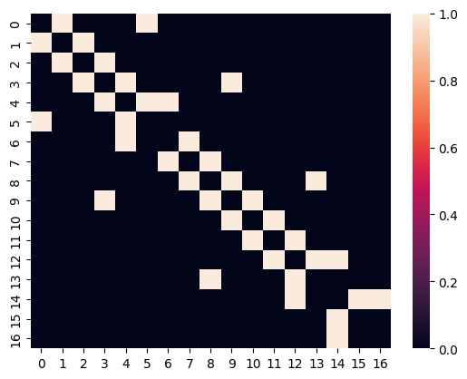
We see it corresponds to an undirected graph, as the adjacency matrix is symmetric; and it is not weighted, as all the values are 1.

Also, the diagonal is zero, so no self-loops.

Molecule visualization

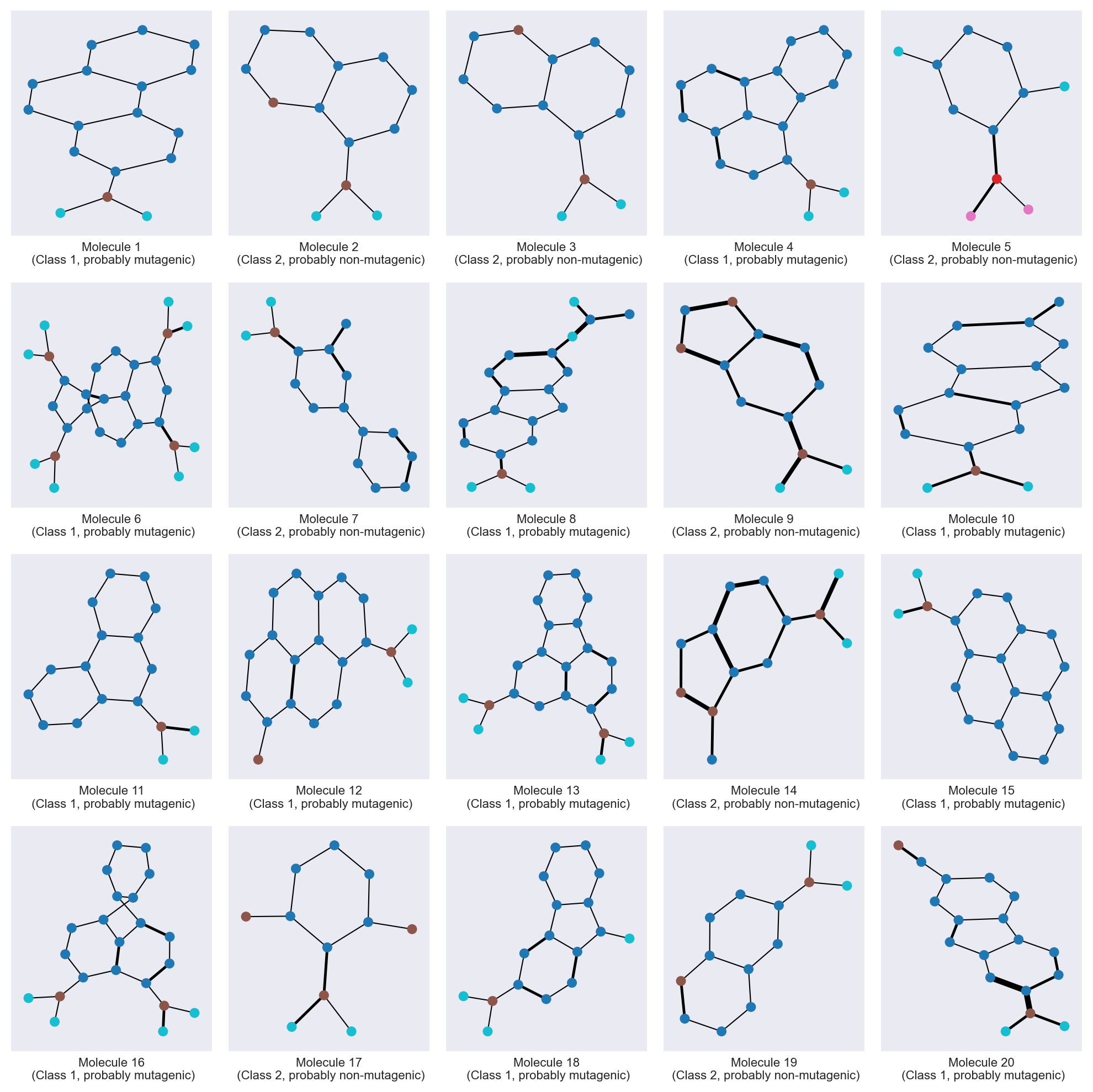
Let’s plot some molecules from the dataset using networkx.

The Kamada-Kawai layout allows to more or less recover a molecule-looking shape, though it is not perfect. We use the atom type for node color, and the edges width is proportional to the bond type.

Show code cell source Hide code cell source

# draw graph of 20 first molecules
_,_ = utils.draw_molecules(
    adjacency_matrices=adjacency_matrices[:20],
    node_features=node_features,
    edge_features=edges_attr,
    class_y=class_y,
)

In the next notebook, we will train a GCN model on this dataset. See Graph Convolutional Network